Google Bigtable as a B-Tree over networked nodes, or - how to scale a database.
Google’s Bigtable is a seminal contribution to database engineering. It was the first database to scale to petabytes of data, and it inspired many of the modern NoSQL databases. In this post, we’ll understand how it scales.
What is a database? A database looks like three things:
- a data structure (table, graph).
- that is language-agnostic to read/write to, through a query language (like SQL).
- that is built for efficient querying (typically using B-Tree’s).
- and is scalable - meaning its capacity can be increased by adding more machines.
The last property - scalability - is the most interesting. How do you scale a database? Or more truthfully, how do you build a distributed data structure?
Review of “scaling” approaches.
There are multiple “approaches” to scaling a database, that fit a business use case. You can split your database by table, and then run the users table on one node and the posts table on another node. This is a manual solution, often referred to as sharding. There is also vertical scaling, which means just buying a bigger machine. But these solutions are manual.
The more automatic solution is described as horizontal scalability. You can add more machines to your database, and the database will automatically split the data across the machines. This is the approach that Google’s Bigtable takes. How does it work?
How does Bigtable scale?
The way I imagine Bigtable’s scaling approach is like applying a binary tree shape to a distributed network.
To begin, imagine an English dictionary for our database table. The keys are the words, the values are the definitions. When we add more words, the dictionary might become too large for a single node to host. So we split the table into two halves - these are called tablets.
A tablet covers a key range. So for example, entries A-L are stored in tablet #1, and entries M-Z are stored in tablet #2. This covers the entire keyspace of A-Z.
Tablets have a fixed capacity, and get split when they become too large. For example, if we added 10,000 new words beginning with A to tablet #1, it might become over capacity and get split. Splitting would produce new tablets, each with smaller key ranges - e.g. tablet #1 of [Aa, Ae], tablet #2 of [Ae, L], and tablet #3 would remain as [L, Z].
Now that we can partition work into equal-sized workloads, it is simple to distribute. We can assign each tablet to a different node, and the nodes can serve read and writes independently. This is the basic idea of Bigtable.
This is why the Bigtable paper describes the tablet as the core unit of load balancing. They begin with the problem - one node cannot handle the entire dataset. They approach the problem approximately - okay, how much can a single node handle? This is the max tablet size/capacity. Then they solve the problem - how do we split the dataset into equal-sized workloads? This is the tablet. Then they distribute the workloads to different nodes.
The detail that is left out is - who orchestrates this process? Who assigns tablets to nodes? Who splits tablets? Who merges tablets? This is the role of the master node.
The master node is responsible for assigning tablets to tablet servers, detecting the addition and expiration of tablet servers, and balancing tablet-server load (splitting/merging tablets).
The binary tree metaphor.
Bigtable can be understood as a B-tree over the keyspace of the dataset, where the leaves are actually database servers. What about the intermediate nodes, how do we actually locate the tablet servers? As in, when we want to RPC call the tablet server to insert a row, how do we actually get the tablet server’s IP address? Remember: we can’t use Bigtable for this, because we’re building Bigtable.
This is an interesting detail of the Bigtable paper.
The intermediate nodes of this tree, except the root, are also stored in Bigtable. The root node, which indexes the intermediate nodes, is stored in Chubby. Since we cannot use Bigtable, we have to store it somewhere.
Chubby is a fixed-capacity data store, built using the Paxos protocol. It is a simpler primitive. Chubby architecture consists of a master node that handles writes, and a set of replicas which serve reads. When the master fails, a new master is elected using the Paxos protocol. Each node serves the same data, and unlike Bigtable, there is no additional storage capacity by adding more nodes.
Chubby’s storage capacity is fixed, but it is actually enough to store enough metadata tablet server locations to make Bigtable work. Let’s work through their calculations.
Each METADATA row stores approximately 1KB of data in memory. With a modest limit of 128 MB METADATA tablets, our three-level location scheme is sufficient to address 2^34 tablets (or 2^61 bytes in 128 MB tablets).
each metadata tablet has a capacity of 128 MB
each metadata row is 1KB
so
  128 MB / 1 KB = 128 000 rows per metadata tablet
  each metadata tablet can address 128 000 user tablets
So each metadata tablet can address 2^17 user tablets (log2(128_000) == 16.9657842847). How much data does the root tablet store? Google described a max addressability of 2^34 tablets, which implies their root tablet stores 2^17 metadata tablet locations, which implies the size of the Chubby file is also 128MB. You might think this is a large file to update over a network, though ask yourself - how often do we need to add a new metadata tablet server? This happens only after 2^17 user tablets have been used. So it is not that often. Plus, Google’s internal data centres have good data transfer speeds.
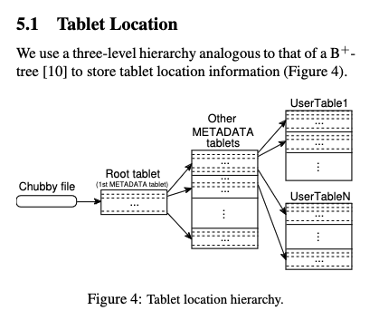
So how does this binary tree look in practice?
root tablet stores     (key range, metadata tablet server location)
metadata tablet stores (key range, user tablet server location)
user tablet stores     (key range, data)

lookup flow to read/write:
  root tablet -> metadata tablets -> user tablets

root tablet      - stored on Chubby
metadata tablets - stored on tablet servers
user tablets     - stored on tablet servers
Why a B-Tree?
A B-Tree is often confused, but it too is easy to understand. A binary tree splits the keyspace into two equal-sized workloads. A B-Tree splits the keyspace into N equal-sized workloads. The N is chosen to maximise the read/write efficiency. This optimization can mean optimizing for the failure rates of hard-drive disk platters (where you only get a certain number of writes - so you want to write as much data as possible in one write), but it can also mean optimizing for minimising network communication of expensive consensus protocols like Paxos. In the case of Bigtable, N = 128 MB so that the root node fits inside a strongly-consistent database called Chubby.
Conclusion.
The purpose of me writing this is to elucidate the simple shapes behind things which seem complex. I am reminded of this Linus Torvalds quote:
programmers worry about the code. Good programmers worry about data structures and their relationships
The Bigtable design is conceptually simple. A large data set is partitioned. How? By splitting the keyspace into equal-sized workloads. We then shape the network into a binary tree, where the leaves are the tablet servers, the intermediate nodes to the leaves are metadata tablet servers, and the root node is stored in another primitive called Chubby.